For my Network Theory I class, I took on a project of designing a simple resistive circuit simulator that takes a user input “netlist”, creates calculations from this “netlist”, and gives back a set of values relating to the current, voltage, and power across each circuit component within the netlist. The circuit simulator that I designed only works with a singular power supply component (i.e. a voltage source or a current source) but works with any quantity or configuration of resistors (technically the math would work with an infinite number of resistors, but computer memory would run out). The calculations that were implemented into the design of this circuit “simulator” were derived from a process called nodal analysis, which is a technique used for solving unknown voltages at certain points within the circuit (called nodes) and using the difference between those points to show the voltage drop across circuit components present between these individual points.
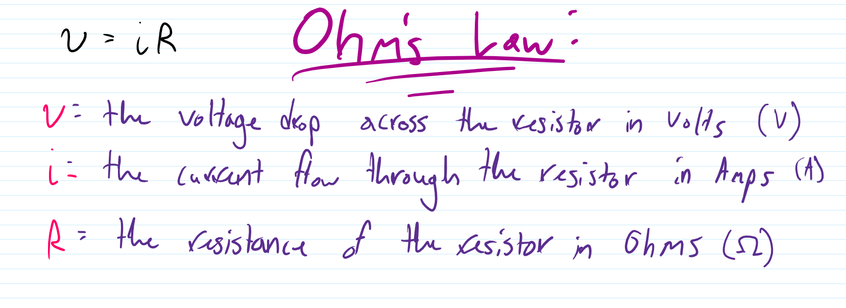
To provide a little more insight into the technique of nodal analysis and what it is, I should first establish some base principles prevalent in circuits and circuit analysis. Certain mathematical laws have been discovered that help describe the relationship between certain behaviors of circuits, the most basic of which is Ohm’s law. Ohm’s law states that the voltage of any component within a circuit is directly related to the resistance of that component multiplied by the current flowing through that component. Ohm’s Law plays a key role with another very important principle when dealing with electronic circuits, Kirchoff’s Current Law (K.C.L.). Kirchoff’s Current Law states that the sum of currents entering and leaving a node (a point that connects two or more circuit components) must equal zero. Manipulation of K.C.L in addition to rearranging Ohm’s law allows us to solve for unknown voltages at the nodes present within a circuit, which is the basis of the technique of nodal analysis.
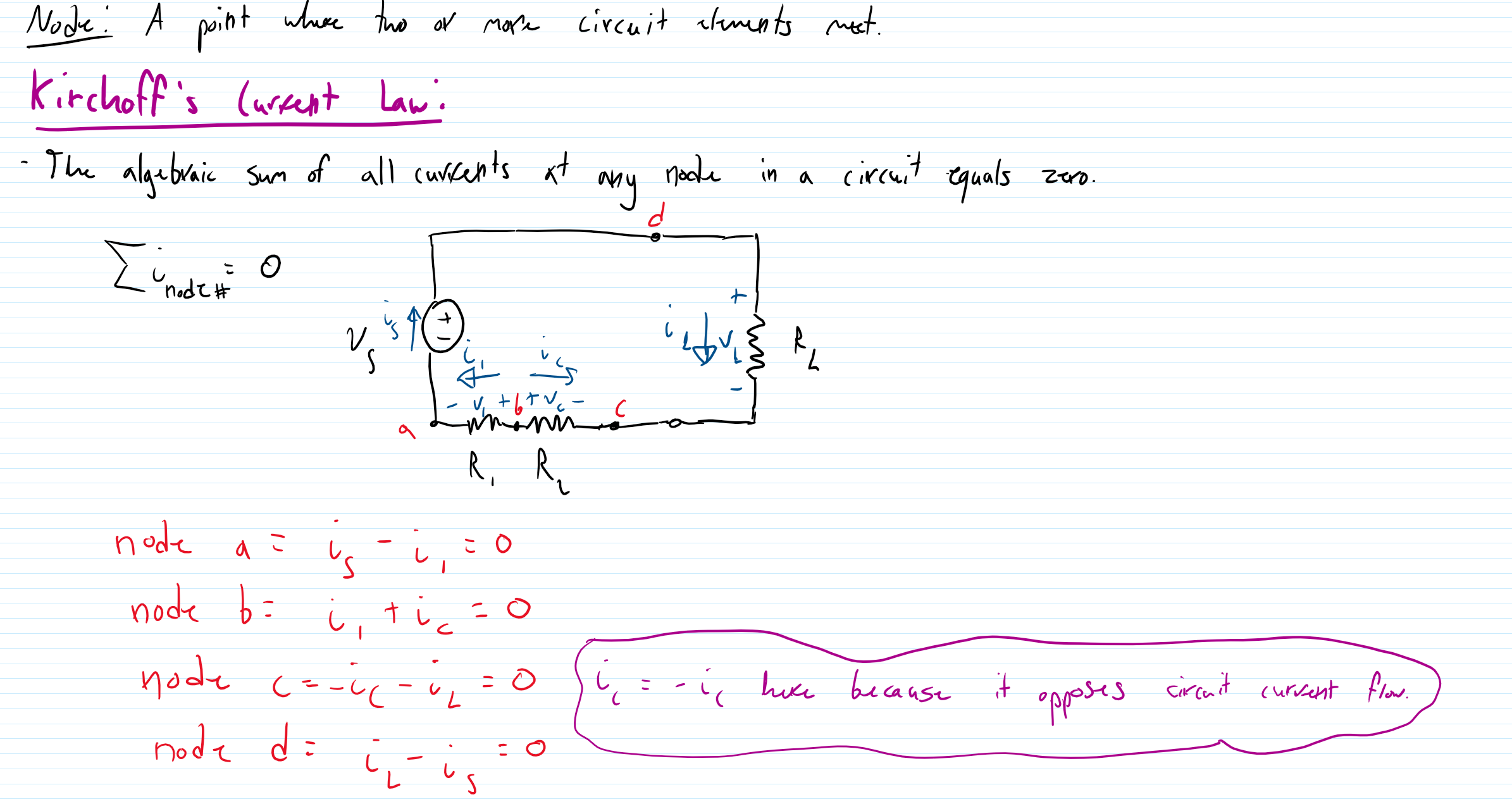
Nodal analysis is a circuit analysis technique that involves writing the current leaving each branch (path of wire) connected to a node as a function of the node voltage and then summing these currents to zero, so that it is within accordance to K.C.L. An example of how this is set up can be seen below:
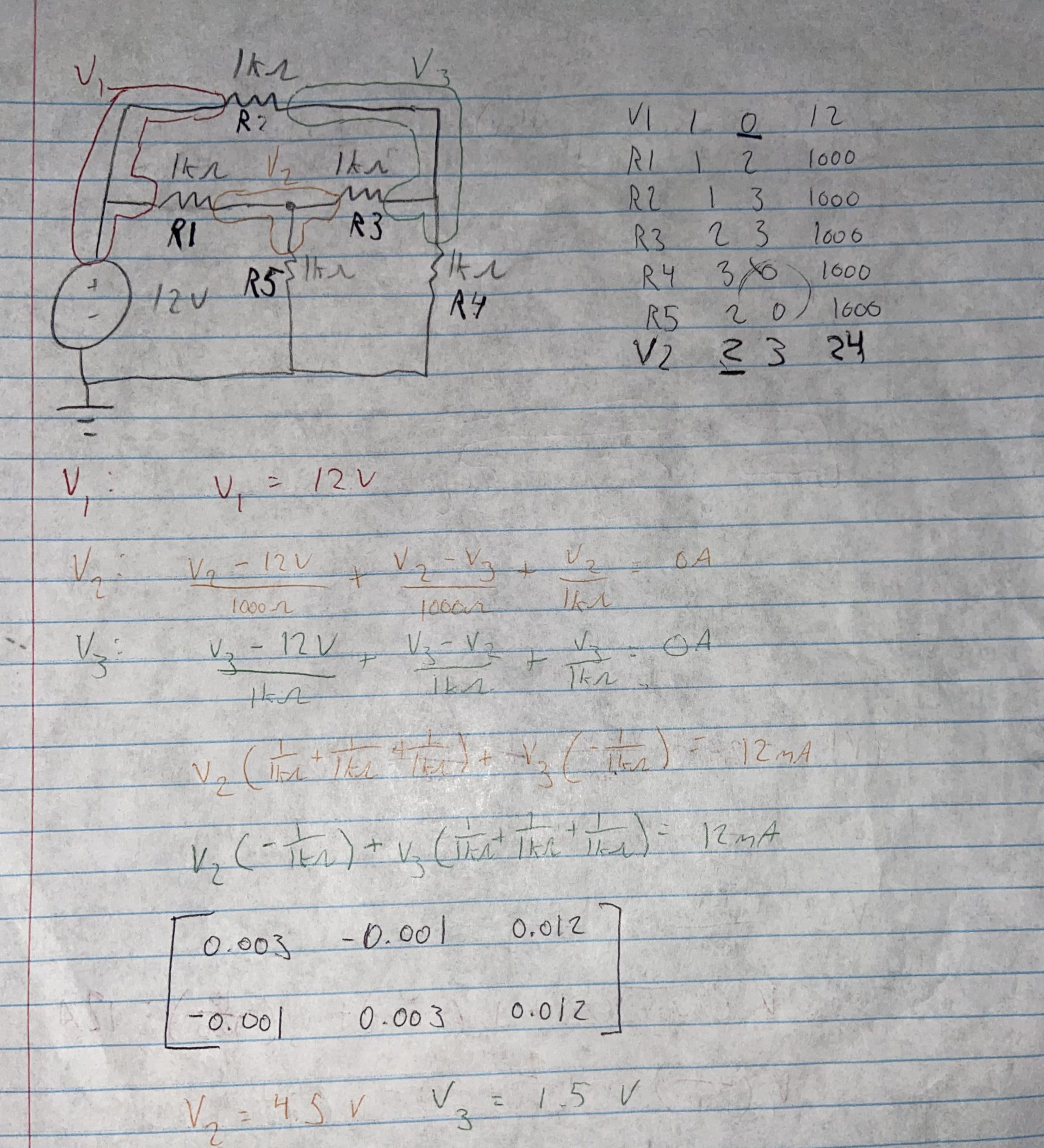
Every node within a circuit thus has an individual equation to solve, so we use linear algebra to accomplish this. By setting equations up in the form:
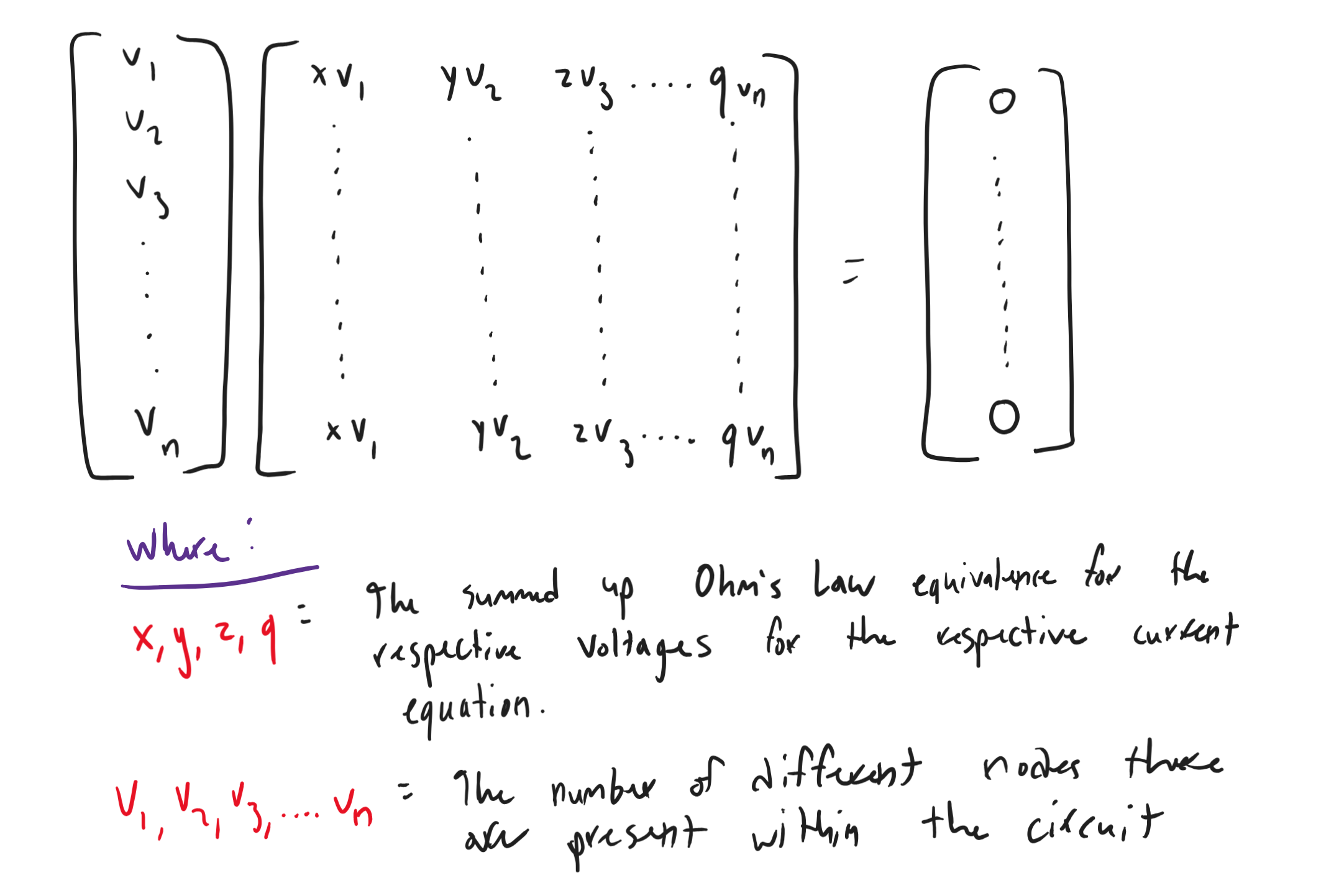
After the individual equations have been set up, we can plug the individual values of each equation into our calculators in a matrix of size Vn x Vn + 1(where Vn represents the number of different nodes that are present within the circuit) and plug in the values of the current column vector (furthest right column labeled above with zeros) into the furthest right spots of our matrix. We can then take our matrix and use a calculation called reduced row echelon form of our matrix (a calculation that is solved within the calculator), which returns the theoretical values of V1, V2, V3….. Vn for every node that we previously defined as being in the circuit. This is essentially all nodal analysis is and it can become very cumbersome to do the more components (therefore the more nodes) you add, which is why it is very helpful to have a computer do these calculations for us.
The process that I used to make Python do these simulations for us is one where I utilized an outside library called numpy, which allows for the creation of the matrix arrays labeled above. The Python interpreter compares the user input values of the netlist at the nodes that they were described as being in, stores the Ohm’s Law equivalence for the respective unknown node voltage for each individual current equation into an equation matrix, and then uses reduced row echelon form to figure out the unknown node voltages. The library that I used to do the reduced row echelon form calculation comes from an imported Python library called sympy, which has a bunch of linear algebra-solving techniques built into it. Python then prints out back into the file that the netlist was created in the voltage, current, and power present at each component by looking at the nodes the component was defined as being attached to, calculating the difference between those nodes, storing that as that components voltage drop, then using the component’s input value to determine current (using Ohm’s law), and multiplies the current by the voltage which returns power (Power = Current x Voltage).
A more in-depth description of the process used by my code to actually do the above-described sequences can be found in the video presentation below:
The code and other information from my actual circuit simulator can be found on my GitHub page, accessed through the below link:
https://github.com/EthaMagn4601/Circuit-Simulator.git
Recent Comments