3D Vector Field Plotter

Coordinate Systems:

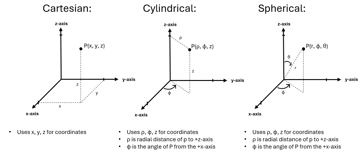
To provide more insight into the behind-the-scenes way this 3D plotter works, I should first establish the concepts behind the different coordinate systems (cartesian, cylindrical, and spherical) and how to convert between them. Starting with the very basics, I’ll define what a point in space is. To define a point in space, the common representation is with the cartesian coordinate system, in which three axes exist: x-axis, y-axis, and the z-axis. These axes are perpendicular (orthogonal) to each other, such that we can represent any point in 3D space as a multiplicative length of one unit on these axes. Similar to how a 2D graph works, 3D graphs (in Cartesian) operate on a notion of being at a point of n number of units along an axis. For example, a point in space could be modeled by (x = 3, y = 2, z = 1), in which that point would exist 3 units in the positive x-axis direction, 2 units in the positive y-axis direction, and 1 unit in the positive z-axis direction. Similarly, with the cylindrical and spherical coordinate systems, the coordinates exist n number of units along the respective standard axes that exist within those systems.  An image depicting how the standard axes are defined in cartesian, cylindrical, and spherical can be seen below:

There also exists a way to convert a coordinate system point to another coordinate system through the definition of how each coordinate point is defined. The standard conversions for these points can be seen in the below image:

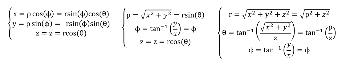
An example of converting from a cartesian point to a cylindrical point can be found if we take (x, y, z) = (1, 2, 3) as our cartesian coordinate point. Through direct substitution of our cartesian values into the equations, we can find that the corresponding cylindrical coordinate point would be (ρ, ϕ, z) = (√5, 63.43°, 3). 

Vectors:

The next component of 3D space that should be defined is the concept of a vector. Vectors are quantities that have both magnitude and direction. In mathematics, physics, and other STEM fields that want to represent some quantity of magnitude and direction, we define vectors as being a straight line from one point to another (giving a magnitude of the vector related to its length between the points and direction given between the difference between those points). We represent vectors similarly to points (as they are two points themselves), by having a standard of axes per coordinate system, called unit vectors, which are perpendicular to each other and have a magnitude/length of 1 in the direction they are defined. This is formally defined as “The unit vector for coordinate 𝜏 points in the direction of increasing 𝜏 and is normal to the surface where 𝜏 is constant”. We use the fact that the magnitude of a unit vector is 1 to define vectors as a composite of the standard unit vectors in a given coordinate system. For example, the vector pointing from the origin (x = 0, y = 0, z = 0) to the point (x = 4, y = 3, z = 5), we would represent the vector in the cartesian coordinate system as being  = 4x̂ + 3ŷ + 5ẑ. 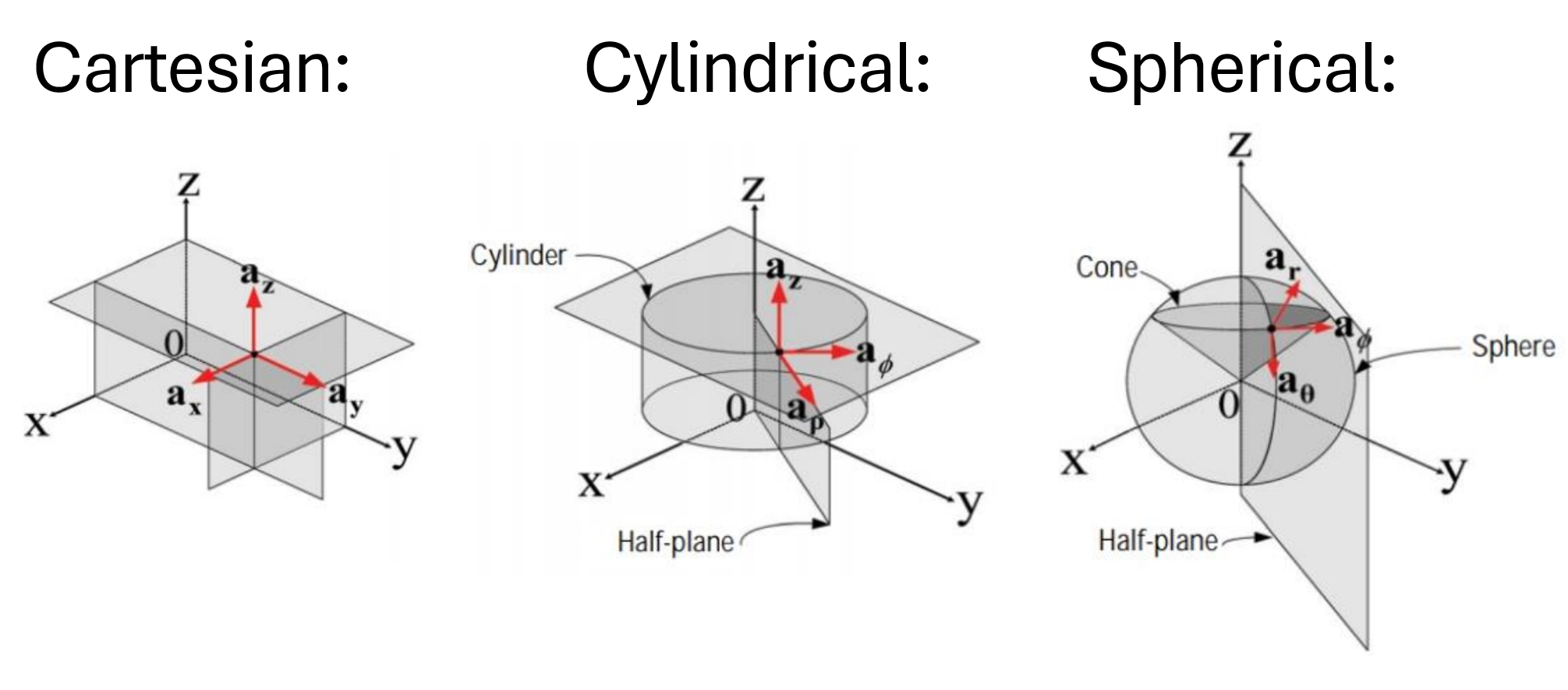The same follows for vectors defined in the cylindrical and spherical coordinate systems, however, due to the definition of a unit vector (that being a vector that always points in the direction of increasing the value that it is representative of), the , , , unit vectors change depending on the position of the vector. The unit vectors are always orthogonal to each other in each coordinate system, they just change their direction depending on where the vector is spatially located. This is a little bit easier to see rather than explain, so I’ve included a picture below depicting how the different unit vectors are represented depending on their coordinate system:

Vector Fields:

I should also distinguish between a vector and a vector field, as this entire project revolves around plotting vector fields, not individual vectors. A vector field is a quantity that has a vector representation for every point in space. This means that for every point in space, we have a defined vector with a magnitude and a direction. For every point within the 3D space, we treat the vector as originating at the point we are analyzing. For example, to plot the vector = 4x̂ + 3ŷ + 5ẑ., we assume that this is with respect to its origin, i.e. (x = 0, y = 0, z = 0), but for a vector field, we assume the origin of the vector to be the point of space that we are analyzing. To put it in other terms, we move the origin to each and every point along the 3D space that we are considering and plot the vector equation, treating the point we are analyzing as being the origin. This is a bit hard to explain without showing a visual representation, so I’ve depicted the vector equation of = 1x̂ + 1ŷ + 1ẑ below:

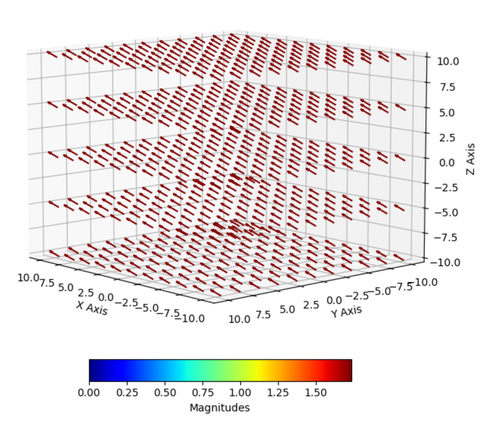
In this example, we can see that all the individual vectors point in the same direction because each vector has a constant magnitude and direction at every point in 3D space. This illustrates how we define a 3D vector field: while the individual vectors are identical (in terms of their magnitude and direction), the origin shifts to be the point in space that’s being plotted. Essentially, the vector field “shifts” the origin to each point in space, so while the vectors themselves remain the same, their positions in space change. A good example of vector fields that change with respect to 3D space are magnetic fields, specifically dipole magnetic fields. As you get further and further away from the origin of a magnetic dipole, the strength of the magnetic field decreases drastically. This can be modeled through the following cartesian equation (try it yourself): = (x*y)/((x**2+y**2)**(5/2)) x̂ + (y**2-x**2)/((x**2+y**2)**(5/2)) ŷ. The resultant vector field is shown below:

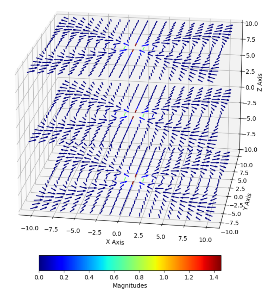
From this 3D plot, we can see that the magnetic field is strongest at the origin (0, 0, 0), denoted by a dark red color, and that as the coordinates in the graph get further away from the origin the magnetic field decreases to practically zero, denoted by a dark blue color.

Vector Coordinate System Transformations: 

Finally, I should introduce vector coordinate transformations and their importance. The vector coordinate systems don’t directly transform into one another due to their different definitions, so special equation transformations must be done to accurately convert a vector to another coordinate system. The transformations that must be used for these conversions can be seen below:

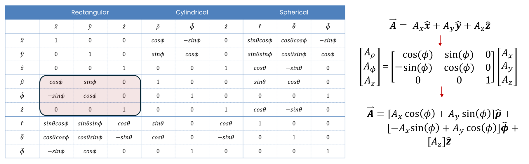
For instance, if we had a vector defined in the cartesian coordinate system, say = 4x̂ + 3ŷ + 5ẑ, the resultant vector in the cylindrical coordinate system would be = [4*cos(ϕ) + 3*sin(ϕ)]x̂ + [-4*sin(ϕ) + 3*cos(ϕ)]ŷ + [5]ẑ.

Now, you might be asking “What’s the purpose?”. The purpose behind using different coordinate systems is to make the math with certain integration techniques a lot easier to compute. Due to the nature of how the unit vectors of the cartesian coordinate system are defined, it is very easy to define boundaries for linear bodies. For example, defining the bounds of a rectangle are rather easy when doing integrals in the cartesian coordinate system. The problem arises (in cartesian) when we try to define anything circular/curved, as this deals with angles, it involves the usage of a lot of trig functions. To combat this problem, the cylindrical and spherical coordinate systems were made to do easier calculations, however, the same problem that occurs with cartesian occurs in both cylindrical and spherical as well. Due to the angular nature of these coordinate systems, it is not easy to define a linear body without the use of a lot of trig functions. This is why the ability to switch between these coordinate systems is so important, to allow for us to simplify some of the expressions that we need to evaluate and make our lives easier when doing certain math operands.

Intro:

Now that we’ve established what vectors, fields, and coordinate system transformations are, I’ll actually start talking about my code. Through this explanation of how the code works, I’ll talk about the main features of the code and how I designed it. As stated at the beginning of my blog post, the libraries that I used for this project were sympy, numpy, matplotlib, and tkinter. To properly utilize this code, you must install sympy, numpy, and matplotlib yourself, otherwise there will be a lot of errors that occur.

The main goals that needed to be reached with the completion of this coding project were, 1.) conversion of a user input vector field to the two other corresponding vector fields, 2.) a working GUI that takes user input of a vector field equation and then displays that vector field equation on a 3D plot, and 3.) a user defined selection between relative vector length and color coding to show relative vector magnitude.

GUI:

The GUI is what mainly comprises the code as it houses all of the information behind the behavior of the plotter. The creation of the GUI utilizes a native Python library called tkinter, which allows for the combination of interactive buttons, text entry fields, windows, and menus to enhance user experience. The way that I designed the GUI to work is by allowing a user to define a vector field equation in a respective coordinate system (coordinate system can be changed through menu button), the view size of the 3D graph (n units * n units * n units), and the number of sample spaces along the ±x-axis, ±y-axis, and ±z-axis. An image of the GUI can be seen below:

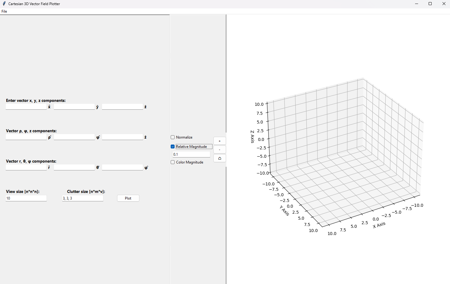
As shown in the picture, I designed the GUI with checkboxes—Normalize, Relative Magnitude, and Color Magnitude—that allow different ways to view the vector field. Selecting Normalize sets all vector lengths equal, showing only directional differences in the 3D plot. Relative Magnitude sets the size of all the vector lengths to their true scaled magnitude multiplied by a user-defined scalar constant. Color Magnitude displays all vector lengths equally, but displays the true magnitude as a certain color corresponding to a magnitude color map. The convention that I chose for the color map was a color map that has its lowest value corresponding to dark blue colors and its highest value corresponding to a dark red color. These different methods for displaying the vector field allow for a better understanding of how the vector field behaves spatially.

Additionally, I included buttons to allow for easier user view-ability, through the use of the zoom buttons located to the left of the plot. The plus and minus buttons zoom in and out, and the home button resets the plot to its original view, making it easier to focus on specific areas and return to the default orientation.

Code Functionality:

Before I begin talking about how the code specifically functions, I want to talk about what the libraries used in this project do. As I said at the beginning of this post, this project uses the outside libraries sympy, numpy, and matplotlib.

• Sympy is a symbolic computation library, that allows for algebraic manipulation of equations and mathematic calculations using symbols rather than numerical values. This library allows for easy computation of equations for variables that are strings, allowing for easy access to simplifying expressions and solving equations. The way that I utilized this library is through the direct substitution of variables into long string equations that arise from the conversions of one coordinate system to another.
• Numpy is a library widely used for numerical computations within Python and is widely used for its usage in multi-dimensional arrays and matrices. This library allows for easy creation and manipulation of large data sets, which is very useful when defining multitudes of coordinate points. This being said, I utilize this library through the creation and usage of every data point that is plotted on the 3D vector plot.
• Matplotlib is a library that allows for the creation of visualization of sets of data through multitudes of 2D & 3D figures. This library allows you to create barcharts, line plots, histograms, piecharts, and many many more types of graphical plots to allow for data representation. I utilize this library through the creation of a certain type of 3D plot, called a 3D quiver plot, in which you can define vector lines as arrows in a 3D spacial grid. This interfaces really well with tkinter, as you can import the 3D quiver plot as a canvas and the plot be interactive in a GUI, so I naturally went with this option to include into my tkinter GUI.

The way that I designed the code to function, was for it to first take the user input of the vector equation and convert the vector into the other corresponding vector coordinate systems (i.e. cart. -> cyl. & spher. or cyl -> cart. & spher.) and display them on the GUI. Regardless of the original coordinate system, the user input vector equation is converted to cartesian for plotting, as matplotlib requires a vector input in terms of cartesian coordinates. Next, user input graph view size and clutter size are used determine the amount of spacial coordinates along the x, y, and z axes, which is calculated based on the view size divided by the clutter size. This defines an array of n columns and 7 rows, that represent all x, y, z, ρ, ϕ, θ, and r values for every cartesian coordinate on the graph.

Each column corresponds to the values defined in the previously defined order (x, y, z,ρ, ϕ, θ, r), for example, column 1 (index 0 in Python) represents all possible x values for all y, z, ρ, ϕ, θ, and r values, column 2 represents all possible y values for all x, z, ρ, ϕ, θ, and r values, etc. This is done to allow for the sympy library to work its magic. The sympy library substitutes all of the possible values of the 3D spacial array into the previously defined user input vector equation, which returns the solved values to the matplotlib 3D quiver plot, which the quiver plot interprets as being the x̂, ŷ, ẑ components (respectively) of each individual vector corresponding to each point on the 3D plot. If there were any previous vector fields plotted, they get cleared and then the new 3D quiver plot is displayed in the 3D plot portion of the GUI. 

I know the explanation behind how the brains of this project work is rather short, especially compared to the code spanning roughly 1000 lines. My goal is to keep things general and accessible, avoiding confusion for readers who may be less familiar with Python or coding in general. Additionally, most of the code is centered around defining parameters for the GUI, which I’ve previously described in the GUI subsection, so I’m trying to avoid reiterating GUI functionality here.